 |
||||||||
 |
 |
 |
 |
|||||
 |
||||||||
 |
||||||||
 |
 |
|||||||
 |
||||||||
 |
||||||||
 |
||||||||
 |
||||||||
 |
||||||||
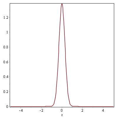
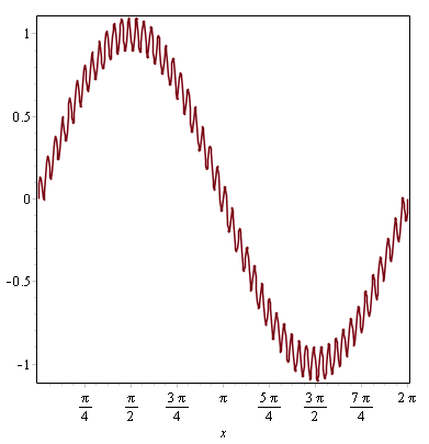
(10) f(x) = sin(x) + 0.1sin(50x)
This function contains two frequencies, one of them being fifty times higher than the other one. You can imagine this function as being the velocity component that needs to be smoothed in LES. As an example, a Gaussian filter was used with different values for Δ. The results are shown in Fig. 2↓. In the first case, Δ = 1 is larger than the wavelength of the small oscillations (λ1 = 2π ⁄ 50≃0.13). The latter are therefore removed from the signal. However, the slower motion has a wavelength λ2 = 2π which is larger than Δ. It follows that only the high frequency oscillations are filtered. In the second case, the value of Δ is very small (10 − 5), well below the wavelengths of all sinusoides. Therefore, both the initial and filtered signals are identical. The exact same concept is applied to the flow field in LES.
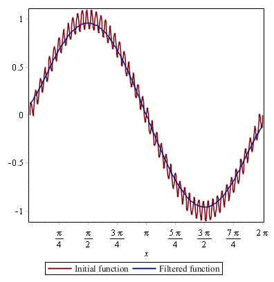
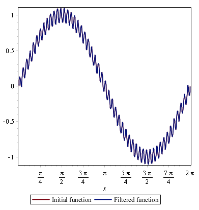
Figure 2
Gaussian filter applied to the function defined in Eq.(10↑). On the left: Δ = 1. On the right: Δ = 10 − 5.
References
[1] K. Sreenivasan. An update on the energy dissipation rate in isotropic turbulence. Physics of Fluids, 10:528, 1998.
← Previous Page
← Previous Page