Algebraic models are the simplest form of turbulence models. The eddy viscosity is described by a basic algebraic relation. This approach was first introduced by Prandtl (1925) with his mixing-length hypothesis. In analogy to the molecular momentum process, Prandtl postulated that for a shear flow moving in the x direction, where the mixing length l_mix depends on the nature of the flow and is typically space dependent. The mixing length model is said to be incomplete. A prior knowledge of the flow is required to obtain reliable results. For example, experimental data suggested that the mixing length of a free shear flow is proportional to the half-width b of the layer. 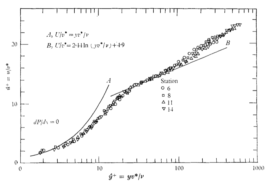Prandtl postulated that the mixing length of a wall bounded flow would be proportional to the distance from the surface. This assumption is consistent with the well known law of the wall, which describes the velocity profile into the log layer. In this region, the flow is sufficiently close to the wall so that the inertial terms can be neglected, but still far enough to neglect the viscous stresses compared to the Reynolds stresses. In a two-dimensional incompressible boundary layer, the Navier-Stokes equations can be written Neglecting the convective terms, the sum of viscous and Reynolds stresses must therefore be constant in the flow completely to the surface, where u_τ = √(τ_w ⁄ ρ) is called the friction velocity. It is frequently used to non-dimensionalize the velocity and distance from the wall, through the equations where y is the distance from the wall and ν is the molecular kinematic viscosity. Introducing Prandtl’s eddy viscosity (l_mix = κy, with κ constant) into Eq.(5↑) and neglecting the viscous stresses, the following equation is obtained. which can be integrated to yield